Euler method

The same idea used for slope fields--the graphical approach to finding solutions to first order differential equations--can also be used to obtain numerical approximations to a solution. The basic idea of differential calculus is that, close to a point, a function and its tangent line do not differ very much. Consider, for example, the function tex2html_wrap_inline49, and its tangent line at tex2html_wrap_inline51 .
Now consider the differential equation
displaymath31
If we want to compute the solution passing through the point (-1,4), then we can compute the tangent line at this point. Its slope at x=-1 is given by the differential equation
displaymath32
thus, the equation for the tangent line is given by
displaymath33
Since we expect the solution to the differential equation and its tangent line to be close when x is close to -1, we should also expect that the solution to the differential equation at, let's say, x=-0.75 will be close to the tangent line at x=-0.75.
We compute the y-value of the tangent line to be y(-0.75)=2.75. This method can now be iterated; the tangent line equation for x=-.075 and y=2.75 is given by
displaymath34
using the tangent line equation for x=-0.5, we obtain as an approximation to our solution
displaymath35
You can use a programmable calculator or a symbolic math program like Mathematica to do the calculations a little faster.
What is the formula we use to find our approximations?
We start at the point tex2html_wrap_inline75 . Let h denote the x-increment. Then tex2html_wrap_inline81 . tex2html_wrap_inline83 is the the y-coordinate of the point on the line passing through the point tex2html_wrap_inline75 with slope tex2html_wrap_inline89 thus tex2html_wrap_inline91
The next approximation is found by replacing tex2html_wrap_inline93 and tex2html_wrap_inline95 by tex2html_wrap_inline97 and tex2html_wrap_inline83 ; so tex2html_wrap_inline101 and tex2html_wrap_inline103 . In general, we obtain the following formula for tex2html_wrap_inline105 ,
eqnarray10
We obtain better approximations if we reduce the step size h. The following graphs give approximations for step sizes h=0.25 in blue, h=0.1 in purple and h=0.01 in red:
For this example it is not hard to compute the exact solution
displaymath36
The next graph shows the exact solution in black. We see that a step size of h=0.01, leading to 500 steps of computation, does a satisfactory job in approximating the exact solution.
The rest of this page is devoted to some of the pitfalls of numerical computations. Here is another example of a "harmless" differential equation:
displaymath37
First, we try Euler's method with a step size of h=0.1. Recall that this step size gave a satisfactory approximation in the previous example.
Not much is happening. Note, however, that the scale on the y-axis is of the magnitude tex2html_wrap_inline121 .
Let's try again with a step size of h=0.0025, leading to 6,000 computing steps.
It is easy to solve the differential equation analytically (do it!). The next picture compares the previous approximation (in red) to the graph of the exact solution (in black). The approximation is off by about 50%!
It is of interest to use numerical methods only when one is unable to compute solutions with pencil and paper. But, in such a situation you cannot compare the approximation to the exact solution so you have no control over how good your approximation is! If you take a course in Numerical Mathematics you will learn that there are ways to predict the error in Euler's method even if you cannot compute the exact solution. The class is also the place to learn more sophisticated numerical methods to solve differential equations. For the differential equation we considered, one should use a method which automatically reduces the step size where the slope of the solution changes rapidly!
The last example addresses another pitfall. Let's consider the differential equation
displaymath38
We want to find the solution satisfying the initial condition y(0)=1.1, using Euler's method with step size h=.1.
The following is a table with the first four values; the function is decreasing rapidly:
displaymath39
Let's look at the graph of the approximation.
The next picture compares the approximation (in blue) to the graph of the exact solution (in red).
Notice that there is no hint of a resemblance between the two. What has happened? An explanation requires the knowledge of the concept of a node. The differential equation has an equilibrium solution y=1. The equilibrium is a down node; thus the exact solution with initial condition y(0)=1.1 is decreasing and approaches 1 as t approaches infinity. The Euler approximation "jumps" below the equilibrium solution in the first computational step (look again at the table above). Once it is below the equilibrium solution it moves away from the position of the node rather rapidly! In our case, a smaller step size would prevent the Euler approximation from ever jumping below the equilibrium solution. 

 reference: www.sosmath.com
» ادامه مطلب

The Perceptron


A Learning Program

For decades there have been attempts to create computer programs that can learn like people - Artificial Intelligence. For example, how do you teach a child to recognize what a chair is? You show him examples telling him "This is a chair ; That one is not a chair" until the child learns the concept of what a chair is. In this stage, the child can look at the examples we have shown him and answer correctly to the question "Is this object a chair?". Furthermore, if we show to the child new objects, that he didn't see before, we could expect him to recognize correctly whether the new object is a chair or not, providing that we've given him enough positive and negative examples. This is exactly the idea behind the perceptron.

The Perceptron

The perceptron is a program that learn concepts, i.e. it can learn to respond with True (1) or False (0) for inputs we present to it, by repeatedly "studying" examples presented to it. The Perceptron is a single layer neural network whose weights and biases could be trained to produce a correct target vector when presented with the corresponding input vector. The training technique used is called the perceptron learning rule. The perceptron generated great interest due to its ability to generalize from its training vectors and work with randomly distributed connections. Perceptrons are especially suited for simple problems in pattern classification. Our perceptron network consists of a single neuron connected to two inputs through a set of 2 weights, with an additional bias input. The perceptron calculates its output using the following equation:
P * W + b > 0
        
where P is the input vector presented to the network, W is the vector of weights and b is the bias.

The Learning Rule

The perceptron is trained to respond to each input vector with a corresponding target output of either 0 or 1. The learning rule has been proven to converge on a solution in finite time if a solution exists. The learning rule can be summarized in the following two equations:
For all i:

                W(i) = W(i) + [ T - A ] * P(i)

                b    = b + [ T - A ]
        
where W is the vector of weights, P is the input vector presented to the network, T is the correct result that the neuron should have shown, A is the actual output of the neuron, and b is the bias.

Training

Vectors from a training set are presented to the network one after another. If the network's output is correct, no change is made. Otherwise, the weights and biases are updated using the perceptron learning rule. An entire pass through all of the input training vectors is called an epoch. When such an entire pass of the training set has occured without error, training is complete. At this time any input training vector may be presented to the network and it will respond with the correct output vector. If a vector P not in the training set is presented to the network, the network will tend to exhibit generalization by responding with an output similar to target vectors for input vectors close to the previously unseen input vector P.

Limitations

Perceptron networks have several limitations. First, the output values of a perceptron can take on only one of two values (True or False). Second, perceptrons can only classify linearly separable sets of vectors. If a straight line or plane can be drawn to seperate the input vectors into their correct categories, the input vectors are linearly separable and the perceptron will find the solution. If the vectors are not linearly separable learning will never reach a point where all vectors are classified properly. The most famous example of the perceptron's inability to solve problems with linearly nonseparable vectors is the boolean exclusive-or problem.

Our Implementation

We implemented a single neuron perceptron with 2 inputs. The input for the neuron can be taken from a graphic user interface, by clicking on points in a board. A click with the left mouse button generates a '+' sign on the board, marking that it's a point where the perceptron should respond with 'True'. A click with the right mouse button generates a '-' sign on the board, marking that it's a point where the perceptron should respond with 'False'. When enough points have been entered, the user can click on 'Start', which will introduce these points as inputs to the perceptron, have it learn these input vectors and show a line which corresponds to the linear division of the plane into regions of opposite neuron response. Here's an example of a screen shot:
Image: Example screen shot
» ادامه مطلب

نانو فناوری


نانو فناوری از فرآیند تصفیه نفت هم بی‌ضررتر است
گروهی از پژوهشگران با مطالعاتی که بر روی مقایسه اثرات زیست محیطی نانو فناوری و دیگر فناوری‌های کنونی داشتند به این نتیجه رسیدند که فرآیندهای تولید نانو موادی مثل کوانتوم داتها (Quantum dots) ، نانو لوله‌های کربنی و باکی بال‌ها(Bucky balls= یک فولرن Fullerene C60 کروی که یک شکل بسیار باثبات از کربن خالص است و از در کنار هم قرار گرفتن متناوب پنج ضلعی و شش ضلعی‌هایی ساخته شده است) نسبت به فرایندهای صنعتی مثل تصفیه نفت، دارای خطرات کمتری برای محیط زیست هستند. در مورد نانولوله‌ها و نانوذرات آلوموکسان (Alumoxane)، خطرات تولید آنها آنقدر اندک است که می‌توان آنها را با فرآیندهایی مثل تولید آسپرین یا شراب مقایسه کرد. این تحقیق که در شماره ماه نوامبر نشریه Environmental Science and Technology چاپ خواهد شد به مقایسه خطرات زیست محیطی تولید پنج نانو ماده (نانو لوله‌های کربنی تک جداره، باکی بال‌ها، کوانتوم دات‌های سلنید روی [Zinc Selenide]، نانو ذرات آلوموکسان و نانو ذرات دی اکسید تیتانیوم) با خطرات تولید شش محصول روزمره (ویفرهای سیلیکونی [Silicon Wafers] ، شراب، پلاستیک فشرده، باتری‌های اسیدی ـ سربی ماشین‌ها، نفت تصفیه شده و آسپرین) می‌پردازد. Mark Wiesner که استاد مهندسی شهرسازی و محیط زیست در دانشگاه رایس (Rice) و یکی از محققان این گروه است، می‌گوید که اطلاعات زیادی در مورد تاثیرات نانو مواد بر روی موجودات زنده و اکوسیستم‌ها وجود ندارد ولی مطالب زیادی در باره ویژگیهای مواد مورد استفاده در ساخت نانو مواد در دست داریم. وی می‌افزاید که هدف آنها از این تحقیق، تخمین اولیه اثرات زیست محیطی تولید نانو مواد بوده است. که این گروه امیدوار است که با انجام این تحقیق بتواند پایه‌ای برای توسعه مسؤلانه و بی‌ضرر صنعت تولید نانو مواد پی‌ریزی کند. در این تحقیق، محاسبه دقیقی از میزان مواد مصرفی، مواد تولیدی و مواد دفعی هر فرآیند صورت گرفت. سپس برای هر فرآیند، خطرات را بصورت کیفی و بر مبنای فاکتورهایی مثل سمیت، آتش‌زا بودن و پایداری در محیط، مورد سنجش قرار دادند. این گروه با استفاده از دستورالعمل‌ تهیه شده توسط شرکت بیمه XLدر زوریخ ، سه نوع خطر را باری هریک از یازده فرآیند مورد مطالعه در نظر گرفتند: خطر حوادث، که به حوادث احتمالی در حین فرآیند می‌پردازد؛ خطر علمیات‌های عادی، که به مواد دفعی می‌پردازد؛ و خطر آلودگی‌های بعدی، که به آلودگی‌های احتمالی در درازمدت می‌پردازد. بنا به گفته Wiesner ، در مورد اغلب فرآیندهای نانو خطرات حوادث قابل مقایسه یا کمتر از خطرات فرآیندهای غیرنانویی می‌باشد. یعنی اینکه خطرات ناشی از تولید مواد نانو تفاوت چندانی با خطرات فناوریهای کنونی ندارد. خطرات عادی علمیاتی فرایندهای تولید نانو لوله‌ها و آلوموکسانها با خطرات تولید شراب و آسپرین قابل مقایسه است در حالیکه خطرات باکی بال‌ها، کوانتوم دات‌ها و دی اکسید تیتانیوم با خطرات عملیاتی تولید ویفرهای سیلیکونی و باتری ماشین برابر می‌کند. ضمنا خطرات عملیاتی تولید پلاستیک و تصفیه نفت بیشتر از خطرات عملیاتی تولید همه نانو مواد می‌باشد. خطرات آلودگی‌های بعدی در تولید همه نانو مواد به استثنای باکی بال‌ها با خطرات آلودگی بعدی در تولید ویفرهای سیلیکونی، شراب و آسپرین برابری می‌کند. خطرات آلودگی بعدی باکی بال‌ها با خطرات تولید پلاستیک و باتری ماشین برابری می‌کند ولی بسیار کمتر از خطرات تصفیه نفت است. پیش‌بینی خطرات احتمالی ناشی از تولید نانو مواد جدید در آینده بسیار دشوار است ولی در وضعیت کنونی می‌توان به این نتیجه رسید که خطرات زیست محیطی ناشی از تولید نانو مواد تفاوت چندانی با بسیاری از صنایع گسترده کنونی مثل ساخت پلی اتیلن با مواد دارویی ندارد.

» ادامه مطلب

تک رقصندگان کائنات


تک رقصندگان کائنات

در سال 1951 شواهدی به دست آمد که رقصندگان آواره ای مشغول نمایش های تک نفره در گستره فضای میان کهکشانی (فضای بین کهکشان ها) هستند ؛ فضایی که تصور می شد صرف نظر از ملکول های اتفاقی و پراکنده گاز و غبار خلأ است. یک اختر شناس سوئیسی به نام فریتز زوییکی گزارش داد که در تصاویرش از خوشه ای از هزاران کهکشان، به نام خوشه گیسو که حدود 350 میلیون سال نوری از زمین فاصله دارد، نوری محو دیده می شود که از خود کهکشان ها ساطع نمی شود. او چنین نظر داد که این نور متعلق به ستاره هایی است که از خوشه رها و به فضای میان کهکشانی پرتاب شده اند.
زوییکی، که همیشه نظریه های عجیب و غریبی از اختر شناسی ارائه می کند که اتفاقا بیشتر اوقات درستی شان ثابت می شود، نتوانست همتایانش را در این مورد متقاعد کند. آنها بر این باور بودند که تصاویر او به علت تغییرات در حساسیت صفحه های عکاسی خراب شده اند.

این موضوع باقی ماند تا اوایل دهه 1970 که کامپیوترهای سریع و پر قدرت در دسترس قرار گرفتند و اخترشناسان از آنها برای شبیه سازی آنچه در تصادم کهکشان ها رخ می دهد استفاده کردند. شبیه سازی ها با اطمینان نشان می دهند که کهکشان های عضو یک گروه یا خوشه کهکشان ها به وسیله کشش گرانشی متقابل قدرتمندشان پس زده میشوند و سرانجام چند تا از آنها با هم برخورد می کنند و کهکشان هایی با اشکال عجیب، معمولا بیضوی، تولید میکنند.
درکمال شگفتی، در طی تصادم تعداد محدودی از ستاره های کهکشان های برخوردی باهم برخورد می کنند چون فضای میان ستاره ای (فضای بین ستاره ها) آنقدر وسیع است که آنها معمولا فقط اثر کشش گرانشی متقابل یکدیگر را از دور حس می کنند و اگر به هم نزدیک شوند ممکن است در مدارهایی به دور یکدیگر بیفتند یا پیش از تصادم از کهکشان بیرون پرتاب شوند.
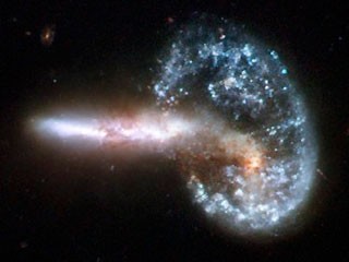
تلسکوپ فضایی هابل نماهای نزدیکی از چند کهکشان برخوردی گرفته است که نشان میدهد در جریان تصادم، ستاره های بسیاری متولد می شوند چون موج ضربه های تصادم باعث فشردگی گاز میان کهکشانی میشود.
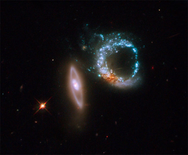
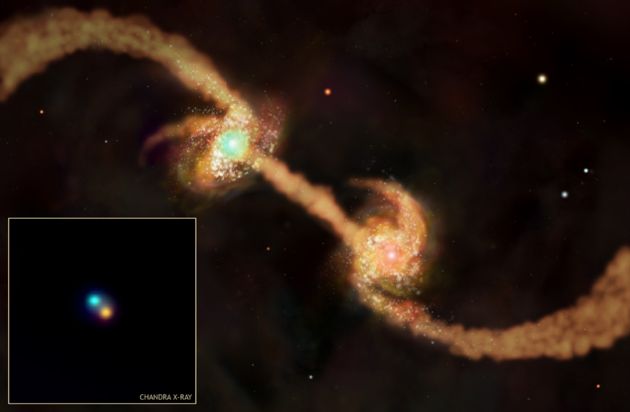
یکی از این کهکشان ها، کهکشان آنتن در واقع نمای دو کهکشان در میانه تصادف به همراه دو رشته از ستاره هاست که از دو سو بیرون زده اند. در حقیقت در سال 1996، شبیه سازی های مشابهی نشان داد که حتی برخی ستاره ها در لبه دو کهکشان که با فاصله دور و با سرعت زیاد از کنار هم میگذرند به فضای میان کهکشانی پرتاب می شوند. این واقعه ای است که باید در خوشه های پر جمعیت و فشرده، همچون خوشه کهکشان سنبله، رخ دهد.
کشف تک رقصندگان کائنات
مندز، کودریتزکی و گروه اخترشناسان همراهشان تصمیم گرفتند نور این سحابی ها را تجزیه و تحلیل نموده تا سرعتشان را محاسبه کنند که ممکن بود به میزان پراکندگی ماده تاریک در M86 رهنمونشان کند. وقتی داده ها را تحلیل می کردند متوجه شدند که سه سحابی بیش از حد سریع، و در جهتی حرکت می کنند که به نظر می رسد متعلق به M86 نیستند. آنچه موجب شگفتی شان شد این بود که دریافتند این سحابی ها در فضای میان کهکشانی خارج از M86، و نه در فضای میان ستاره ای داخلش قرار دارند.
در همین حال، اخترشناسان اهل توسان انگلستان که به رصد سحابی سیاره نمایی در M86 ، کهکشان بیضوی غول پیکر دیگری در خوشه سنبله، مشغول بودند متوجه شدند که بیشتر آنها درخشان تر از آن اند که انتظار داشتند. پس از چند ماه برایشان روشن شد که این ها می بایست نسبت به بقیه بسیار نزدیک تر به زمین باشند – آنها می بایست در فضای میان کهکشانی قرار داشته باشند.
کمی بعد اخترشناسان موسسه تلسکوپ فضایی گزارش دادند که با استفاده از تلسکوپ فضایی هابل حدود 600 ستاره غول سرخ (ستاره های پیری که هنوز موادشان را فوران نکرده اند یا منفجر نشده اند ) را در فضایی خالی در آسمان نزدیک M86 یافته اند.
پس از اینکه اخترشناسان انگلیسی اعلام کردند که آنها هم ده سحابی سیاره نما در فضای میان کهکشانی خوشه کور، در گوشه ای دیگر از عالم یافته اند، دیگر شکی نبود که بی شمار ستاره های درخشان و بقایای تعداد بیشتری ستاره مرده در این بخش فضا پراکنده اند، البته این که دقیقا این مقدار بی شمار چقدر است هنوز مطمئن نیستیم.
رصد بخش های مختلفی از فضای میان کهکشانی خوشه سنبله نشان داده که جمعیت غول های سرخ و سحابی ها در بعضی قسمت ها کمتر از بخش های دیگر است. بنابراین، تخمین جمعیت کلی ستاره های میان کهکشانی در کل خوشه فقط بر اساس چند رصد محلی امکان پذیر نیست. افزون بر این، تخمین جمعیت همه انواع ستاره ها با شمارش غول های سرخ و سحابی های سیاره نما مثل این است که جمعیت شهری را از روی افراد پیر و سنگ قبرهای قبرستان شهر تخمین بزنیم. با این همه، اخترشناسان جمعیت ستاره های فضای میان کهکشانی یک خوشه از کهکشان ها را حدود 20 تا 100 درصد جمعیت ستاره های کهکشان های آن خوشه تخمین می زنند.
نوشته شده توسط خانم شیما نامی
» ادامه مطلب

تصویر بسایر زیبای ایستگاه فضایی در مقابل ماه


ایستگاه فضایی بین‌المللی در ارتفاع 400 کیلومتری از سطح زمین به دور سیاره مادری در گردش است و شبانگاهان می‌توان آن را به شکل نقطه‌ای نورانی مشاهده کرده که به آرامی از غرب به شرق آسمان را درمی‌نوردد.
اما بعضی وقت‌ها پیش می‌آید که این ابزار بزرگ که هم‌اکنون وسعتش از یک زمین فوتبال هم فراتر رفته، از مقابل ماه یا خورشید بگذرد و چشم‌اندازی جالب را پدید آورد.
این تصویر نیز به هنگام عبور ایستگاه فضایی بین‌المللی از مقابل ماه گرفته شده است.


» ادامه مطلب

dictionary

به اشتراک بگذارید